A kosarad üres
Oktatási szoftverek
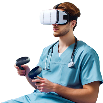
mozaMedical
Digitális, komplex tananyag az egészségtudományi képzéshez.
Az egészségtudományi ismeretek elmélyítéséhez és a tudás ellenőrzéséhez használd a mozaMedical STUDENT licencet, ha tanórán vagy konferencián prezentálni szeretnél esetleg alacsony sebességű internet eléréssel rendelkezel, akkor válaszd a mozaMedical PRESENTER licencet. Intézményi kedvezményekért keresd munkatársunkat!
mozaMedical - Digitális, komplex tananyag az egészségtudományi képzéshez
mozaMedical PERSONAL
Diákoknak - tanuláshoz, gyakorláshoz
- Hozzzáférsz a digitális leckékhez
- VR szemüveggel és anélkül is gyakorolhatod az oktatási szimulációkat
- Bármilyen eszközzel használhatod.
XR Extended Reality
99 EUR / Felhasználó
Felhasználó

mozaMedical PROFESSIONAL
Oktatóknak - oktatáshoz, prezentációkhoz
- Lenyűgöző kurzusok egy gombnyomásra
- Interaktív ellenőrző eszközök
- Nagyképernyős előadások tanórán és konferenciákon
XR Extended Reality
198 EUR / Felhasználó
Felhasználó
*Licenc PACK: a PACK csomagban vásárolt licencek egy közös aktiváló kóddal rendelkeznek, amellyel annyi helyen lehet aktiválni a szoftvert, ahány licencet tartalmaz a csomag.
Felhasználói licenc
A felhasználói licenc segítségével a felhasználó különböző eszközökön (számítógépen, interaktív táblán, notebookon, tableten, mobilon) jelentkezhet be a saját azonosítójával. Mind a mozaBook, mind a mozaWeb rendszert használhatja, de egy időben csak egy eszközről tud bejelentkezni. Abban az esetben javasolt, amikor a felhasználók saját eszközökön dolgoznak, vagy több eszközön is hozzá szeretnének férni a Mozaik-rendszerhez.
Eszközalapú licenc
Az eszközalapú licenc segítségével az adott eszközön a szoftvert korlátlan számú felhasználó használhatja. Ilyen esetben a felhasználóknak nem szükséges licenccel rendelkezniük. Abban az esetben javasolt, amikor egy eszközt több tanár vagy diák használ. Ennél a licencnél csak az eszközöket kell licencelni, függetlenül attól, hány tanár vagy diák fér hozzá. Vásárlás előtt elfogadandó jogi nyilatkozat
A School Admin Licenc megvásárlásával kijelentem, hogy:
- Az intézmény kifejezett megbízásából vásárolom meg a licencet, és kizárólag az intézmény nevében, annak hivatalos céljaival összhangban fogom használni.
- Tudomásul veszem, hogy a licenc jogellenes használata, különösen ha személyes adatokat jogosulatlanul kezelek, az bűncselekménynek minősül.
- Büntetőjogi felelősségem tudatában kijelentem, hogy a vásárlás során minden jogi és etikai felelősséget vállalok, és tisztában vagyok vele, hogy bármilyen jogellenes cselekedet, különösen a felhasználói adatokkal való visszaélés, jogi következményekkel jár.
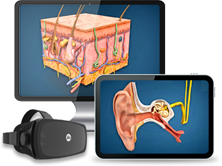
cadaVR - Digitális anatómia atlasz

cadaVR PERSONAL
Diákoknak - tanuláshoz, gyakorláshoz
- Felhasználói licenc, amellyel egy diák több eszközön is használhatja a digitális anatómiai atlaszt.
- Teljes hozzáférés az interaktív tartalmakhoz, feladatokhoz, VR funkció (PC VR) használatához.
XR Extended Reality
Licenc Pack*
99 EUR / Felhasználó
Felhasználó

cadaVR PROFESSIONAL
Előadóknak - oktatáshoz, prezentációkhoz
- Felhasználói licenc, amellyel egy előadó/orvos több eszközön, projektoron, illetve interaktív táblán is használhatja a digitális anatómiai atlaszt.
- Teljes hozzáférés az interaktív tartalmakhoz, feladatokhoz, VR funkció (PC VR) használatához.
- Gyorsabb működés, kevesebb adatforgalom - letölthető 3D modellek az adatforgalom csökkentése céljából.
XR Extended Reality
Licenc Pack*
198 EUR / Felhasználó
Felhasználó
*Licenc PACK: a PACK csomagban vásárolt licencek egy közös aktiváló kóddal rendelkeznek, amellyel annyi helyen lehet aktiválni a szoftvert, ahány licencet tartalmaz a csomag.
Felhasználói licenc
A felhasználói licenc segítségével a felhasználó különböző eszközökön (számítógépen, interaktív táblán, notebookon, tableten, mobilon) jelentkezhet be a saját azonosítójával. Mind a mozaBook, mind a mozaWeb rendszert használhatja, de egy időben csak egy eszközről tud bejelentkezni. Abban az esetben javasolt, amikor a felhasználók saját eszközökön dolgoznak, vagy több eszközön is hozzá szeretnének férni a Mozaik-rendszerhez.
Eszközalapú licenc
Az eszközalapú licenc segítségével az adott eszközön a szoftvert korlátlan számú felhasználó használhatja. Ilyen esetben a felhasználóknak nem szükséges licenccel rendelkezniük. Abban az esetben javasolt, amikor egy eszközt több tanár vagy diák használ. Ennél a licencnél csak az eszközöket kell licencelni, függetlenül attól, hány tanár vagy diák fér hozzá. Vásárlás előtt elfogadandó jogi nyilatkozat
A School Admin Licenc megvásárlásával kijelentem, hogy:
- Az intézmény kifejezett megbízásából vásárolom meg a licencet, és kizárólag az intézmény nevében, annak hivatalos céljaival összhangban fogom használni.
- Tudomásul veszem, hogy a licenc jogellenes használata, különösen ha személyes adatokat jogosulatlanul kezelek, az bűncselekménynek minősül.
- Büntetőjogi felelősségem tudatában kijelentem, hogy a vásárlás során minden jogi és etikai felelősséget vállalok, és tisztában vagyok vele, hogy bármilyen jogellenes cselekedet, különösen a felhasználói adatokkal való visszaélés, jogi következményekkel jár.
Intézményeknek - Komplett megoldás oktató intézmények részére

INTÉZMÉNYI licenc
- Intézményi szintű hozzáférés, amellyel egy egészségügyi oktatási intézmény, anatómiai intézet vagy orvosi centrum minden oktatója, diákja, munkatársa teljes körű hozzáférést kap.
- Teljes hozzáférés az interaktív tartalmakhoz, feladatokhoz, VR funkció (PC VR) használatához.
- Gyorsabb működés, kevesebb adatforgalom - letölthető 3D modellek az adatforgalom csökkentése céljából.
Felhasználói licenc
A felhasználói licenc segítségével a felhasználó különböző eszközökön (számítógépen, interaktív táblán, notebookon, tableten, mobilon) jelentkezhet be a saját azonosítójával. Mind a mozaBook, mind a mozaWeb rendszert használhatja, de egy időben csak egy eszközről tud bejelentkezni. Abban az esetben javasolt, amikor a felhasználók saját eszközökön dolgoznak, vagy több eszközön is hozzá szeretnének férni a Mozaik-rendszerhez.
Eszközalapú licenc
Az eszközalapú licenc segítségével az adott eszközön a szoftvert korlátlan számú felhasználó használhatja. Ilyen esetben a felhasználóknak nem szükséges licenccel rendelkezniük. Abban az esetben javasolt, amikor egy eszközt több tanár vagy diák használ. Ennél a licencnél csak az eszközöket kell licencelni, függetlenül attól, hány tanár vagy diák fér hozzá. Vásárlás előtt elfogadandó jogi nyilatkozat
A School Admin Licenc megvásárlásával kijelentem, hogy:
- Az intézmény kifejezett megbízásából vásárolom meg a licencet, és kizárólag az intézmény nevében, annak hivatalos céljaival összhangban fogom használni.
- Tudomásul veszem, hogy a licenc jogellenes használata, különösen ha személyes adatokat jogosulatlanul kezelek, az bűncselekménynek minősül.
- Büntetőjogi felelősségem tudatában kijelentem, hogy a vásárlás során minden jogi és etikai felelősséget vállalok, és tisztában vagyok vele, hogy bármilyen jogellenes cselekedet, különösen a felhasználói adatokkal való visszaélés, jogi következményekkel jár.
Licencek összehasonlítása - mozaMedical
| PERSONAL LICENC | PROFESSIONAL LICENC | |
| LISTAÁR (1 licenc / év) | 99 EUR / Felhasználó |
198 EUR / Felhasználó |
| Licenc PACK / év (minimum 10 licenc) | 89 EUR / Felhasználó |
178 EUR / Felhasználó |
| Licenc PACK / év (minimum 30 licenc) | 84 EUR / Felhasználó |
168 EUR / Felhasználó |
| Licenc PACK / év (minimum 100 licenc) | 79 EUR / Felhasználó |
158 EUR / Felhasználó |
| Előfizetés típusa | Felhasználói licenc | Felhasználói licenc |
| Hány felhasználó használhatja? | egy | egy |
| Hány eszközön használható? | több | több |
| Elérhető funkcionalitás | PERSONAL | PROFESSIONAL |
| Interaktív tábla / Projektor / Nagy méretű kijelző (30”-nál nagyobb) | ||
| Virtuális valóság eszközök támogatása / PC VR | ||
| Oculus Quest 2 | hamarosan | hamarosan |

Felhasználói licenc
A felhasználói licenc segítségével a felhasználó különböző eszközökön (számítógépen, interaktív táblán, notebookon, tableten, mobilon) jelentkezhet be a saját azonosítójával. Mind a mozaBook, mind a mozaWeb rendszert használhatja, de egy időben csak egy eszközről tud bejelentkezni. Abban az esetben javasolt, amikor a felhasználók saját eszközökön dolgoznak, vagy több eszközön is hozzá szeretnének férni a Mozaik-rendszerhez. |
||